
모두를 위한 딥러닝 강의 시즌1을 듣고 복습한 내용입니다.
Classification
- 스팸 메일 찾기: 스팸 or 스팸X
- 페이스북 피드: Show or Hide
=> 0, 1 encoding
- 스팸 메일 찾기: 스팸 (1) or 스팸X (0)
- 페이스북 피드: Show (1) or Hide (0)
Linear Regression으로 표현했을 때 애매한 경우
- 공부 시간 당 합격할지 예측
- 합격(1), 탈락(0)
데이터의 수, 종류에 따라 linear 선이 달라짐

50시간 공부한 데이터가 추가되었을 때는 기울기가 낮아지면서, 데이터를 대표하지 못하게 된다.
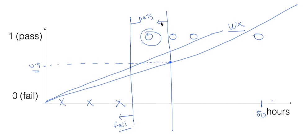
기존 가정
H(x) = Wx + b가 데이터를 잘 나타내주지 못함 => 새로운 함수를 사용해야 함
- 시그모이드 함수


그러나, 그냥 Sigmoid 함수를 사용하면 문제점이 있다.

Sigmoid함수 사용 시 Global minimum이 아니라 Local minimum을 찾아버릴 수 있다.
따라서 약간 변형해서 사용해야 함
=>

다시 복습해보면,
예측값과 비슷하면 Cost는 0에 가깝게
예측값과 멀었다면 Cost는 크게 계산되야 한다.
y = 1이 목적일 때는 위에 식
y = 0이 목적일 때는 밑의 식을 쓰는 것이다.
1. y = 1이 목적일 때 ( 1인 라벨을 찾는 것일 때 )
H(x) = 1일 때가 맞는 것이므로 cost를 계산해보면 0
H(x) = 0일 때는 틀린 것이므로 cost를 계산해보면 무한대
2. y = 0이 목적일 때
H(x) = 1일 때가 틀린 것이므로 cost를 계산해보면 무한대
H(x) = 0일 때는 맞는 것이므로 cost를 계산해보면 0
코드로 if문 쓰는 거 불편하니까 식을 좀 변형하면 다음과 같다.

텐서플로우 코드 (버전 2.0 이상)
import tensorflow as tf

x_data = [[1, 2],
          [2, 3],
          [3, 1],
          [4, 3],
          [5, 3],
          [6, 2]]
y_data = [[0],
          [0],
          [0],
          [1],
          [1],
          [1]]

tf.model = tf.keras.Sequential()
tf.model.add(tf.keras.layers.Dense(units=1, input_dim=2))
# use sigmoid activation for 0~1 problem
tf.model.add(tf.keras.layers.Activation('sigmoid'))

'''
better result with loss function == 'binary_crossentropy', try 'mse' for yourself
adding accuracy metric to get accuracy report during training
'''
tf.model.compile(loss='binary_crossentropy', optimizer=tf.keras.optimizers.SGD(lr=0.01), metrics=['accuracy'])
tf.model.summary()

history = tf.model.fit(x_data, y_data, epochs=5000)

# Accuracy report
print("Accuracy: ", history.history['accuracy'][-1])
2
import tensorflow as tf
import numpy as np

xy = np.loadtxt('../data-03-diabetes.csv', delimiter=',', dtype=np.float32)
x_data = xy[:, 0:-1]
y_data = xy[:, [-1]]

print(x_data.shape, y_data.shape)

tf.model = tf.keras.Sequential()
# multi-variable, x_data.shape[1] == feature counts == 8 in this case
tf.model.add(tf.keras.layers.Dense(units=1, input_dim=x_data.shape[1], activation='sigmoid'))
tf.model.compile(loss='binary_crossentropy', optimizer=tf.keras.optimizers.SGD(lr=0.01),  metrics=['accuracy'])
tf.model.summary()

history = tf.model.fit(x_data, y_data, epochs=500)

# accuracy!
print("Accuracy: {0}".format(history.history['accuracy'][-1]))

# predict a single data point
y_predict = tf.model.predict([[0.176471, 0.155779, 0, 0, 0, 0.052161, -0.952178, -0.733333]])
print("Predict: {0}".format(y_predict))

# evaluating model
evaluate = tf.model.evaluate(x_data, y_data)
print("loss: {0}, accuracy: {1}".format(evaluate[0], evaluate[1]))'딥러닝, 머신러닝 > 모두를 위한 딥러닝 강의 복습' 카테고리의 다른 글
| Learning rate, Data preprocessing, Overfitting, Regularization (0) | 2022.01.07 |
|---|---|
| Softmax Regression (0) | 2022.01.06 |
| TensorFlow로 파일에서 데이터 읽어오기 (0) | 2022.01.04 |
| Multi-variable linear regression (0) | 2022.01.04 |
| Linear Regression의 cost 최소화 알고리즘의 원리 (0) | 2022.01.04 |